Jane Student
April 26, 2001
Lab Exercise #1: Spatial
Analysis of a survey on attitudes about Population Growth In Santa Barbara County
Assessing ‘Representativeness’ of the survey respondents (1-6)
1)
Were the home locations of the respondents to this survey spatially
random?
(you don’t have to do the analysis on this question, just answer it, & explain how you would have done the analysis if you had to)
No.
This can easily be seen from a quick glance at the data. The respondents are obviously clustered in population
centers. However, if you really wanted
to test this, you could perform a Chi square test through creating an expected
value in a defined area (such as a 1km2 block). You could then divide the total number of
respondents by the number of 1km2 blocks to get an “expected” value
for the x2 test. If the actual number of respondents in a block differs
significantly from an expected number (which it obviously will) then the
locations are random.
2) Were the home locations of the respondents to this survey random with respect to population density? (You do have to do the analysis for this one)
According to a chi squared test, the home locations of
the respondents of the survey were not spatially random with respect to
population density. The formula for
performing the chi-squared is
x2 = Σ(O-E)
2
E
Where O is the number of Observed and E is the Expected
number of samples you should get. The
observed and expected values were obtained by gently massaging the data in
excel and then convincing Bill Gates accounting baby to perform the x2
test. I already gave you the gory
details (lab instructions) so here are the results.
x2 = 281.09235.
p>.05 = 101.9 at 82 degrees of freedom (df from # of
tracts)
Conclusion: We
are 95% confident that the data is not spatially random.
3)
What level of spatial aggregation (tracts or block-groups) is more
appropriate to answering question #2. Explain.
Tracts are more appropriate for determining the spatial
randomness with respect to population.
Tracts are relatively divided by equal population, whereas, blocks are
not. An assumption of this chi square
test is that the spatial areas are equal in population. Block-groups do not
meet this assumption.
4)
How would you test the following?: a) Is the age distribution of the
respondents to this survey significantly different than the age distribution of
the population of
(a &b) To
compare the distribution values for the respondents and county a series Normal
Distribution values can be calculated, such as Standard Deviation, Mean, Mode,
Median. If the values are significantly different, then the distribution is
significantly different.
(c&d) These are spatial distribution questions. A Chi-squared test will test the spatial
randomness of the survey results against the spatial distribution of the County
as a whole. One would have to create an
expected value throughout the county, tracts could be used as in question
3.
5)
What kinds of problems do you run into when trying to answer the
questions posed in #4?
The income distributions from the surveys were based on
ranges. So, the data does not reflect
exact incomes, but a range. The
intervals were standardized into categories for analysis. Non continuous, in this case interval data,
does not fit the normal distribution assumption of the chi squared test or
comparing means and standard deviation.
6)
Are the respondents to this survey age and income independent? Would
you expect them to be? Is this a
parametric or non-parametric test?
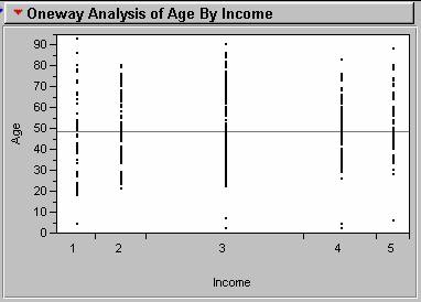
A one-way analysis can by performed in JMP. This analysis differentiates a continuous Y variable against groups defined by a categorical X variable. This initially plots age against income as seen below.
For a
more complete evaluation of non-parametric data, a Tukey Test can be
performed.
The results (below) indicate that there are significantly different (independent) means between age and income. This analysis shows that a younger or older person and their income are independent or significantly different (positive values), whereas, the middle ages tend to be more income dependent (negative values). While one would expect age and income to be dependent, this result could be due to a poor sample of the older and younger population.
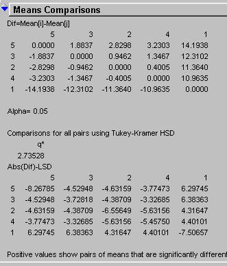
The test was a non-parametric test because the Income
Levels were grouped in Intervals and delineated as Nominal data. Parametric tests are based on intervals and
ratios.
Simple Demographic Comparisons
(7-11)
7)
Based on the responses to the question: ‘Abortion should remain
legal as defined in “Roe v. Wade”?’; are Democrats significantly more
‘Pro-Choice’ than Republicans?
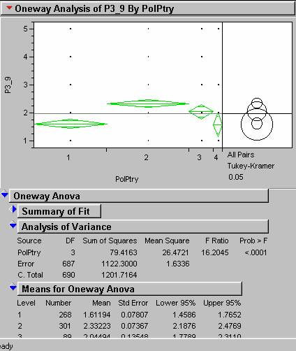
This is simply done by completing a test of Anova in
JMP. Comparing the abortion question
(Page3 No 9), and the Political Party.
The results (below) show that we
can state with 99% confidence that there is a significant difference between
republicans and democrats on the abortion.
8)
Along a similar vein, are Women more ‘Pro-Choice’ than Men? (according
to this survey)
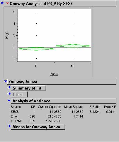
With the same test as 7, only with the SEX as the X
variable, the results (below) show that
women are more ‘Pro-Choice’ than men with 95% confidence.
9)
In a separate survey I found that Women were more ‘Pro-Choice’ than men
and that Catholic women were significantly ‘More, more Pro-Choice’ than
Catholic men. Is this true of the respondents to this survey? How did you test that? If you did find the gap between Catholic men
and women significantly greater than the gap between men and women in general
what would a statistician call such a phenomena? If it were true, how would you
explain it?
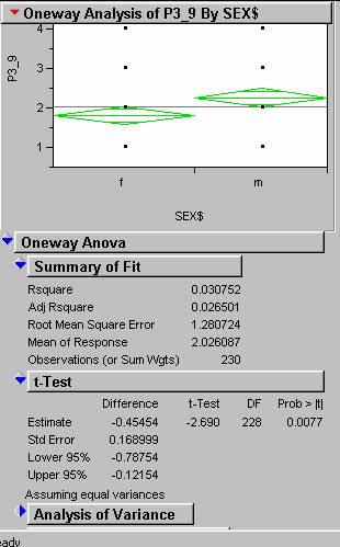
By creating a subset of just
Catholics, we can again perform an Analysis of Variance.
The results (below) of the
Analysis show that there is a 0.7% chance of making a wrong assumption that
there is a significant difference.
Therefore, we can say with 99% confidence that Catholic women are
significantly more ‘Pro-Choice’ than Catholic men.
10)
Are republicans different than non-republicans on the responses to any
of the questions about immigration?
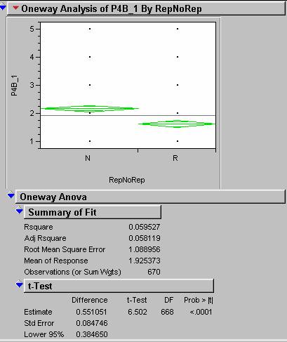
By creating a new column
indicating republican or non-republican we can again evaluate using Anova. The
results (below) show that we can say with 95% confidence that Republicans have
a significantly different opinion on the issues of immigration than
Non-republicans.
11)
Is there any relationship between ‘Religiosity’ and responses to the
question: ‘The earth has a finite supply of natural resources such as water,
arable land, etc. which imposes a limit on the number of people which can
sustainability live on it.’
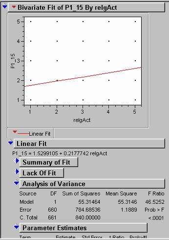
These data are both continuous, so I performed a
Bivariate Analysis. The results below show there is a significant difference of
99.99% confidence that people who are minimally to somewhat active
religiously have a stronger belief (strongly agree to agree) with the question.
However, people who are more religious (some to average) feel the
opposite.
Factor Analysis (12-14). Factor analysis is a data reduction technique that allows you to ‘compress’ your analysis. As you can imagine we could ask hundreds, if not thousands of questions of this dataset (e.g. are men different than women on questions 1-50, are Catholics different than protestants on questions 1-50, there’s a hundred right there). However, as you can imagine, people will have similar responses to many of the questions. Factor analysis allows you to capture the co-variance that usually exists between questions. For example, there are 5 questions about immigration or immigration policy; an anti-immigration person will most likely respond in a similar manner to all the questions and only one question is often necessary to ‘capture’ such a response. Factor analysis is a means of ‘capturing’ this co-variance between questions and ‘reducing’ a many-question survey to a few factors. Labeling or ‘Naming’ these factors is one of the ‘arts’ of statisticians. It is now your turn to practice this ‘art’.
12)
Run a factor analysis on the responses to the questions appropriate to
such an analysis (we’ll decide these in class). Identify the questions
with a factor contribution score of 0.40 or more for each factor and list the
questions associated with factors 1-5. Be sure to save each respondent’s factor
scores on each of Factors 1-5. For Factors 1-5 list the questions with a factor
contribution score of 0.40 or more and study the questions that contributed to
each factor. As a result of this study provide a name for each of the first
five factors. (FYI, potential ‘names’ for factors when I analyzed this survey
were: “Faith in Government”, “Belief in Adam Smith’s ‘invisible hand’”, and
“Keep those Mexicans out of California”). Try to come up with your own (it’s
actually kind of fun J).
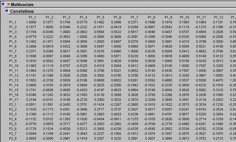
A multivariate principal components/factor analysis was
performed in JMP. This returned a matrix
with all the rankings of each question. A significant result on this matrix has
a ranking of above 0.4 or below -0.4.
From this, I reviewed the questions that had significant rankings for
each factor and grouped them according to the basis of the questions.
The results (below) can be summarized as:
Factor 1: Government should help the helplessly stupid.
P1 (5, 13, 16), P2 (10, 11, 12, 14), P3 (1, 4, 5, 7, 9, 10, 13)
Factor 2: Yuppies don’t like immigrants. P3 (2), P4B (1, 2, 3, 4)
Factor 3:
Californicate the world. P1 (2, 4, -10, -11, 14), P2 (3, 5, 6, 7), P3
(-9, 10, 12)
Factor 4:
Californication is the devil, but the government is God. P1 (1, 3, 5, 6,
7, 9, 10, 11, 12, 13,15) P2 (2, 3, -6)
Factor 5: We want
Chinese population control (didn’t like that 2nd kid anyway). P1
(10, 11), P2 (2, 3, -4) P3 (3, 6, 7, 11, 13, 14)
13)
Do all the statistical tests necessary to fill out the table below. Put
an asterisk (*) in the cells that indicate any significant differences on
factor scores between demographic variables. For each asterisk provide a
detailed description of the nature of the significant differences and some
guess as to an explanation for the differences. Your ‘guess’ is referred to as
‘theory’ in academia. If you are really fired up about this exercise find
references to support your theory.
|
Significant Factor Score
Differences (*) |
Sex |
Pol. Party |
Religion |
Religiosity |
Income |
Education |
Race/Ethnicity |
|
Factor1: |
*0.0029 |
*0.0001 |
*0.0018 |
0.1435 |
0.2010 |
0.5877 |
0.1250 |
|
Factor 2: |
0.3688 |
*0.0001 |
0.0596 |
0.5597 |
0.4762 |
0.0529 |
0.7328 |
|
Factor3: |
0.8586 |
*0.0007 |
*0.0012 |
*0.0001 |
0.3298 |
*0.0005 |
*0.0459 |
|
Factor4: |
0.6749 |
0.8896 |
0.4372 |
0.1071 |
*0.0400 |
0.4943 |
0.5038 |
|
Factor5: |
*0.0448 |
0.3580 |
*0.0301 |
*0.0001 |
0.4673 |
0.2603 |
0.0999 |
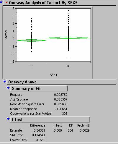
The significance of each factor and
each category in the table was tested using a series of Anova tests. A sample result from the significance anova
analysis is shown below.
14)
Did filling out the table and answering the questions of #13 make you
appreciate factor analysis? (Explain. If
your answer is ‘No’ stop by my office for a spanking J).
I like naming the factors, it is a pitiful means towards
creativity for stats geeks. The table
was a useful way to draw meaning out of my creative license.
Spatial Analysis: Where’s the Geography?
So far, the analyses performed up to this point could have been done in a sociology department. The only ‘geographic’ analyses were the questions about randomness of the survey respondents with respect to population density and space. True spatial analysis of surveys can shed light on interesting questions about the location of the respondent’s home or workplace relative to questions in the survey. For example: Does the distance of a respondent’s home and/or work location influence their likelihood to support or use a light rail public transportation system? Does the population density of their home location or home city covary with attitudes about population growth and policy? Does the Hispanic proportion of their home neighborhood have any influence on their attitudes about U.S. immigration policy?
14) Test for any significant differences/variation for all of the factor scores (1-5) and the population density and percent non-white of the respondents home location. If you find any significant differences provide an explanation?
Factor 3, non-white/white, with a p = 0.0462 was the only case where there was a
significant relationship, meaning non-whites did not agree as much with whites
regarding the questions in factor 3 (named Californicate the world). This is interesting because it shows that the
largely Hispanic population is very much in favor of population growth. The non-significance of the other factors
could be explained by a relative similarity between income and education in the
Santa Barbara area. People of similar income and education levels usually feel
similarly about many issues. In this
case the similarities are represented by the lack of significance between
percent non-whites, whites and population density.
Population Density and Factors
1 0.1420
2 0.5187
3 0.3550
4 0.1010
5 0.9089
%
White/Non-white and Factors
1
0.2033
2
0.8910
3
0.0462
4
0.5962
5
0.1910
15) Another test you could do is to test for increases variance in response based on a geographic attribute. For example, suppose that people’s responses to the 5 immigration questions became increasingly extreme (i.e. more 1’s (strongly agree) and 5’s(strongly disagree)) but the mean remained the same as the Hispanic proportion of the population in the respondent’s home location increased. What kind of statistical test would you use to look for that and if it proved significant, what would the explanation be?
In order to compare variances of the total population and the Hispanic population, you would perform a F-test. If it proves significant, this would mean that there was a significant difference in the variances of the responses between the two groups. This would mean that one group would have “more extreme answers” to the questions.
General Questions
16) Describe 10 specific problems related to this little research project. Things to consider: Sampling frame was registered voters whereas census data was total population, Non-response Bias, etc.
1)
Sample size, is it
representative of the population?
2)
Non-response bias, were
the lazy people a significant cohort, changing results?
3)
Are registered voters
representative of the general population?
4)
Is the census data
representative of the general population?
5)
Were the fill in
questions too vague?
6)
Were responses to fill
in questions biased toward obvious answers?
7)
Were the responses to
the SA-SD questions biased toward extreme answers?
8)
What about the interval
nature of the responses, you can’t run parametric tests, can you?
9)
Is Santa Barbara really
anyplace to do a survey, aren’t they all rich hippies?
10) Did Paul’s dad fudge the data just so his son wouldn’t make
him suffer through all the same crap after a failed survey?
17) Are these problems significant enough to invalidate any or all of the findings from an analysis of this data?
No, the sample size was
sufficiently significant, non-biased, and large enough. Besides, most tests are tests of means, not
individual responses. The central limit
therom validates all these tests.