Jane Doe Spatial Statistics 2001

Lab Exercise #3: Spatial Interpolation: Inverse Distance Weighting and Kriging of Several Datasets including Ozone concentration.

Background

In this lab you will use Arc/INFO (or ArcView if you can find the Avenue scripts to do it) to perform some spatial interpolations on various datasets. You will use two kinds of spatial interpolation: Inverse Distance Weighting (IDW) and Kriging.

Specific Instructions for Tasks 1-4

Outline 1) Do a single IDW calculation by hand and describe how the Grid function IDW does a whole lot more.

Task #1: Inverse Distance Weighting by hand

The table below represents x and y coordinates of something called ‘Value’. Estimate the value of the fourth record (indicated by a ‘?’) using inverse distance weighting. Draw a crude scatter plot of the data in the space to the right of the table.

X coord	Y coord	This calculation by hand shit is out of control. We know computers are fast and powerful. Give me a break. IDW can be done with this formula: Σ (Value /d^2 ) / Σ(1/d^2 ). If you want to see the fractions involved, here it is: Σ(11 / 2^2 + 3 / 17 + 7 / 2^2 + 9 / 17) = 5.2 = 8.5 Σ(1 / 2^2 + 1 / 17 + 1 / 2^2 + 1 / 17) 0.6 Value
1	3	11
3	5	7
2	7	3
3	3	?
7	4	9

?= 8.5

Now, enter this table into Excel or some text editor and read it in as an ‘event theme’ to ArcView. Convert that shapefile to an Arc/INFO point coverage and do an IDW on that point coverage. How did the output of Grid’s IDW command differ from your simple hand calculation? Explain.

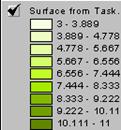
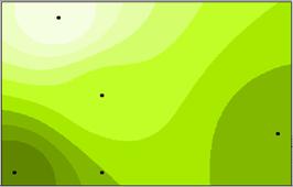
X coord	Y coord	Value
1	3	11
3	5	7
2	7	3
3	3	8.4
7	4	9

The difference is that the information is calculated for every cell; each to every. The answer from the ‘do it by hand’ section is the calculation for just the one missing value. The IDW function calculates the cell values based on the parameters given and uses neighboring points to estimate the value of each cell based on the weight assigned to the distance between the unknown cell and its neighbors. The farther away a known value is the less it matters to the value of the estimate for that cell. Lather rinse repeat. IDW makes these calculations for every cell from every known point or according to limits set by the geographer. The shape of the interpolation window, its radius, and direction of travel across the grid can affect the values assigned to the new grid.

Outline 2) Your second task will be to simply take a point coverage of ozone measurements made throughout the United States and spatially interpolate a grid from these points using both IDW and Kriging. You will then display these two different interpolations and comment on the differences between them. You will also look at the error grid or variance output of the Kriging command.

Task #2: Kriging and IDWing without a ‘truth’ or reference grid

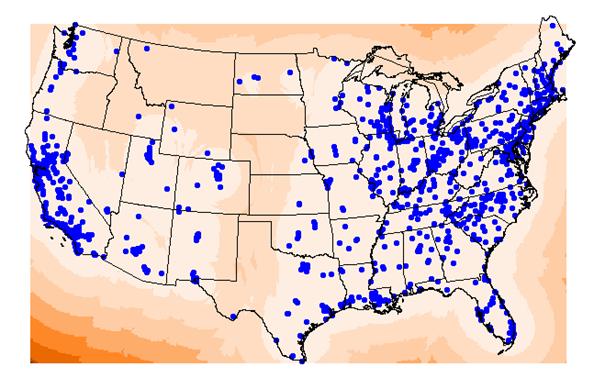
If you look at the Point Attribute table for the point coverage ‘usozonesites’ (usozonesites.pat) you will find that there are numerous attributes. We will work with the attribute: ‘O3apr2oct_’ (don’t forget the underscore ‘_‘at the end). First we will create an interpolated grid of the ‘O3apr2oct_’ values using the Inverse Distance Weighting command. Get into the right workspace and get into Grid. At the Grid prompt type:

Grid: idwozone = IDW(usozonesites, o3apr2oct_,. #, 2, Sample, 11, 1000000, 10000)

Take a look at the grid you created ‘idwozone’ in ArcView. Now create another interpolated filed using the ‘kriging’ command in grid. At the grid prompt type:

Grid: krigozone = kriging(usozonesites, o3apr2oct_,. #, both, varozone, linear, sample, 11, 1000000, 10000)

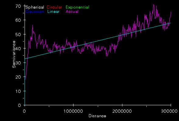
This command produced three things: 1) a kriged estimate of the ‘3apr2oct_’ attribute of the usozonesites point coverage, 2) A semi-variogram of that attribute of the point coverage, and 3) a variance of the kriged estimate grid. To look at these outputs read the interpolated grid ‘krigozone’ into ArcView. Also read the interpolated grid ‘varozone’ into ArcView. To see the semi-variogram run Arcplot, do a disp 9999, then type semivariogram krigozone.svg. This should display a semi-variogram in the ArcPlot display. Use Snag-it to save this image somewhere.

Questions for Task #2:

1) Read the three grids (idwozone, krigozone, and varozone) and a co-registered state boundary coverage into ArcView. Compare and contrast the appearance of these three grids.

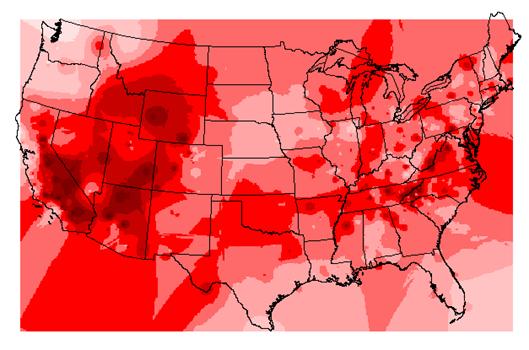
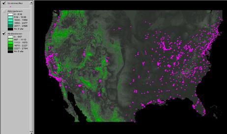
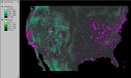
The red IDW image is the interpolation of ozone readings from the point locations. It is calculated by inverse distance weighting. In general it agrees with the kriged estimate shown in purple below. The kriged map also shows the point locations. Kriging uses the varogram to influence the estimate according to the trends in the data. This variogram has a relatively large nugget and small slope with a huge residual variance. These things do not indicate high reliability for the estimate.

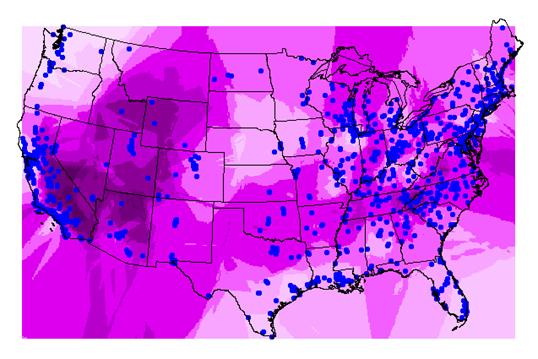
The wavefront varozone (below) is the estimate for each grid cell based on the semivariogram.

2) Where are the areas of high ‘ozone’ concentration in idwozone and krigozone? Do the two images agree in general? Yes. They seem to agree in the areas where point coverage is more dense and vary where there is more distance between points. High concentrations of ozone in the southwest, the mountain west and the central Appalachian mountains do not seem to be correlated to point locations. Each technique interprets the edges differently.

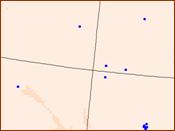3) What is the IDW and Kriged estimate of o3apr2oct_ at the Four Corners location? What is the value of varozone at Four Corners? If the varozone value is the standard error of the estimate of the kriged ozone estimate, what is your 95% confidence interval for the o3apr2oct_ for Four Corners?

Varozone = 37.34

Krigozone = 41.30

IDW = 41.87

95% confidence interval

31 - 53

The confidence interval is determined by using the varozone value = 37.34, taking the square root = 6, multiply by 1.96 then add and subtract that from the krig value. You get a range of 24 centered around the value of 41.30. This range actually exceeds the range of the data. According to reliable sources, a wide confidence interval indicates a lousy ability to guess correctly.

For example; the possibility of throwing a pencil at the wall with 95% confidence of success is much greater than the possibility of throwing the same pencil at the same wall and making it land on the ledge of the blackboard.

Outline 3) One problem with the IDW and Kriging exercises in task #2 is that you can’t really assess how good or bad your interpolations were. So in this third task you will take a complete grid of three datasets (a DEM of the U.S., a landcover grid of the U.S., a population density grid of the U.S) and sample them at the points of the Ozone monitoring stations used in task #2. (You will need to add ‘z’ values from those grid to the usozonesites coverage using ‘summarize zones’ command in spatial analyst of ArcView). You will then produce four kriged and four IDW’d estimates of Elevation, Landcover, population density, and rainfall. You will then look at the errors of these estimates and discuss.

Task #3: Spatial interpolation with a known full valid coverage to validate estimates against

In this task you will be IDWing and Kriging interpolated grids from data you already have ‘truth’ for. To do this you will artificially blind yourself by getting elevation, population density, and landcover information at only the usozonesites points and then interpolating them. To do this you will need to do a ‘summarize zones’ command with ArcView using usozonesites and each of the following three grids: nademlza, uspopden, and naigbplza. This will generate several tables which you will have to read into excel, delete most columns, (keep ‘Monitor’ and ‘Median’), change name of median to elevation, popden, and landcover as appropriate, and join these three tables back to usozonesites.pat. Now you are ready for spatial interpolation.

The Elevation dataset

Get an IDW and a Kriged interpolated grid from the usozonesites pointcoverage from grid

Grid: idwelevation=IDW(usozonesites, elevation,. #, 2, Sample, 11, 1000000, 10000)

Grid: krigelevation = kriging(usozonesites, elevation,. #, both, varelevation, linear, sample, 11, 1000000, 10000)

Questions

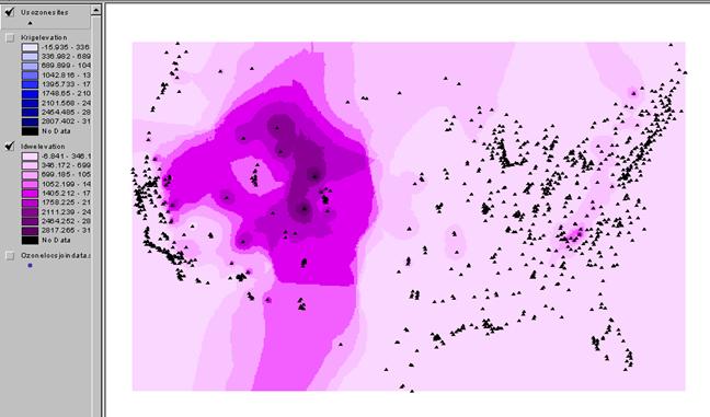
1) Look at these interpolated fields. How well did IDW or Kriging spatially interpolate elevation?
The rockies are dark and the plains are light in both methods. Neither one has much in the way of accuracy. Of course the points are less than random, so clustering of the data may have something to do with it.

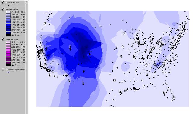
Above: the kriged interpolation surface.
Below: the IDW method.

2) Does the varelevation grid seem honest with respect to characterizing the error of estimate?

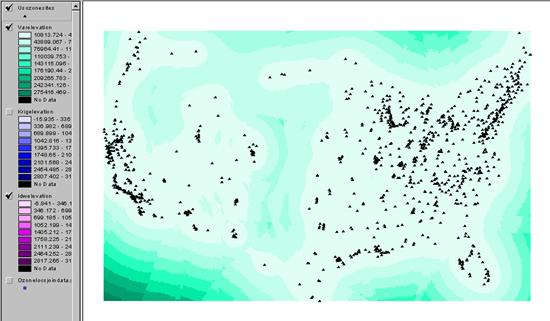
The variance (above) indicates, of course, that the proximity to measurement location has a strong affect on the similarity of the estimate in each of the two methods.

3) Create two error grids with simple map algebra, from grid the commands would be:

Grid: idweleverror = nademlza – idwelevation

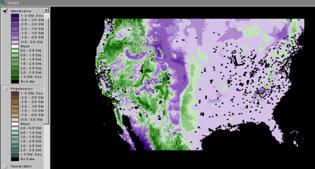
Grid: krigerror = nademlza – krigelevation

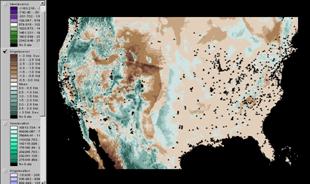
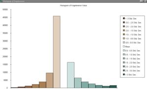
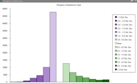
Display the grids idweleverror and krigeleverror in ArcView using standard deviation as a classification and color scheme. How similar are the error patterns?
Very similar patterns at this scale. The over estimated areas and the underestimated areas appear to be in the same locations and the histograms show nearly identical shapes with small differences in absolute count.

4) Now create the absolute error (so over and underestimates do not cancel each other out when you calculate the mean). To do this use the absolute value function in grid:

Absidweleverror = abs(idweleverror)

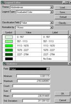
Abskrigeleverror = abs(krigeleverror)

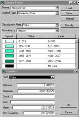
Which interpolator had the lowest Mean Absolute Deviation? Krig: 289

IDW: 311

5) Comment on the usefulness of IDW and Kriging for interpolating Elevation data with point coverages of the density of usozonesites.

It is helpful to have measured locations scattered more evenly throughout the area. As the vast majority of elevation surfaces are generated by interpolation techniques of one kind or the other, the data points should be systematically located to provide the best chance of accuracy. In the case of elevation, it might be good to use elevation at stream gaging stations as the low points and the watershed divides as the highpoints. Elevation is not random.

The Population Density Dataset

Using the population density dataset for the conterminous United States that you used in the nighttime satellite imagery lab repeat the same routine you did with elevation for population density.

Questions 1-B thru 5-B same as elevation dataset

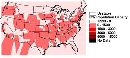
1) Look at these interpolated fields. How well did IDW or Kriging spatially interpolate popdensity?

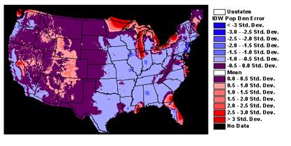
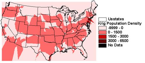
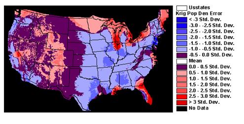
IDW and Kriging cannot do a good job interpolating population because it is not autocorrelated.

2) Does the varpopden grid seem honest with respect to characterizing the error of estimate?
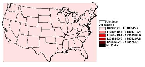
The variance is completely flat because kriging cannot estimate the population.

3) Create two error grids with simple map algebra, from grid the commands would be: see above.

4) Now create the absolute error (so over and underestimates do not cancel each other out when you calculate the mean). Which interpolator had the lowest Mean Absolute Deviation? IDW = 368 Krig = 467. The lower error is the better estimate, even though neither one does a very good job.

5) Comment on the usefulness of IDW and Kriging for interpolating elevation data with point coverages of the density of usozonesites.

Ozone locations are generally more dense in areas with higher population. The problem is that interpolation is used to estimate a single variable with more than one controlling factor. It is better to give more thought to the locations of data stations so that the estimates can be more accurate. If you want to estimate population, you need to have more point locations.

The Landcover Dataset

Using the landcover dataset naigbplza dataset for the conterminous United States was in the nighttime satellite imagery workspace repeat the same routine you did for elevation for landcover.

Note: smart students will not do this and explain to me that it is an inappropriate exercise.

The land-cover data is categorical. That is to say that the number representing each type has no relationship to the number assigned to the other types; grassland is not for example twice as nice as forests. So repeating the routine that worked for continuous data will only cause trouble. It can be done with dummy variables, but that is ‘too much trouble’.

6) Print the variograms for elevation and population density on a sheet of paper side by side. How do they compare and how can they be interpreted in light of what you know about the spatial variability of population and elevation in the conterminous United States.

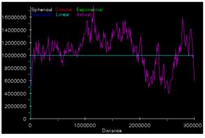
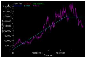
Semivariogram of population density Semivariogram of elevation

The variogram is supposed to be random because population density is highly variable throughout the area of analysis. Isolated spikes of large numbers constitute the statistical surface of the United States population. The variogram of elevation is closely correlated at short distances and random at large distances because elevation is a continuous variable and because landforms are large enough to have spatial autocorrelation.

Outline 4) Build a ‘detrended’ kriged estimate of ozone in Great Smoky NP and compare to U.S. estimate and discuss method.

Task #4: De-Trended Kriging of Ozone in Rocky Mountain National Park

Space is not the cause of variability in measurements of elevation, ozone concentration, etc. Kriging, IDW, and other spatial interpolaters merely take advantage of the fact that spatial auto-correlation exists. It is even better to build a model using spatially explicit measure of dependent variables, apply them to extensive spatial coverages, look at the errors at known points and only krig the errors. Approaches like this are sometimes called ‘de-trended’ kriging. For example, let’s consider ozone concentration in Great Smoky Mountain National Park.

Suppose you have a point coverage of ozone measurements AND that you want an interpolated field.

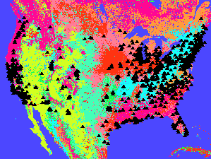with landcover categories.

Suppose you have a DEM, slope, and a land-cover database.

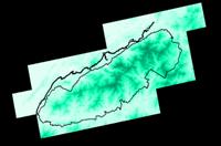
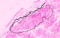
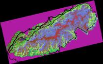
By intersecting the point coverage with these grids (summarize zones in ArcView and a bunch of table joins) you will have a table from which you can build a single or multiple regression to predict ozone from elevation and/or landcover and/or slope. Then apply this regression to those grids.

Compare this ‘model’ to the point values and get ‘errors’ at those point values.

Krig the ‘error’ values at those points and add the interpolated field of errors to your ‘model’.

Compare this to a simple ‘kriging’ and simple ‘IDWing’ of the original point data.

Procedures:

Produce a simple kriged estimate of ozone:

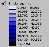
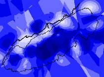
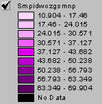
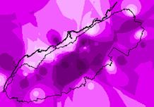
Grid: smpkriggsmnp = kriging(ozonelocs, adj_intsv_, # , both, varsmpkrig, linear, sample, 5, 500000, 200)

Produce a simple IDW estimate of ozone:

Grid: smpkriggsmnp = IDW(ozonelocs, adj_intsv_, #, 2, Sample, 5, 500000, 10000)

Now you need to gather the data needed to build a model that uses more than simply the spatial relationships of the ozone measurements at the ozone monitoring sites. To do this you need to read in the ozonelocs point coverage, and the following grids: gsmnpelev, gsmnp_slope, gsmnp_landcover. Do the GIS manipulations necessary to get a table with the following fields and appropriate values in the records: Code4_site, Elevation, Adj_intsv_, gsmnpelev, gsmnp_slope, gsmnp_landcover. Read that table into JMP.

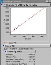
How does the Elevation variable correlate with the gsmnpelev variable? This should be a strong relationship. It’s not perfect because the elevation measurements were made with different devices.

Now build a univariate or multivariate model that predicts Adj_intsv_ using the other variables.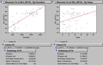

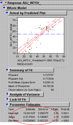Two graphs above show that the two variables seem to have a pretty weak relationship to the dependent variable ‘Y’. The graph on the right shows that the combination of elevation and slope are strongly related to the ozone readings at most locations with an r2 of 0.72.

Build a grid of that model estimate with ArcView or Arc/INFO’s Grid module.

Adj_intsc_ = 10.64 + 0.5137 (slope) + .0257 (elevaton)

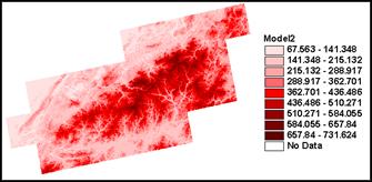
Questions:

1) How do these models compare visually? The multivariate model takes more factors into account and produces a model that is closer to reality than the interpolated versions.

2) How could you quantitatively compare the accuracy of these interpolations?
Subtract the estimate from the data and find the errors. Krig them to get a surface that you can combine with the estimate to correct the estimate.

-for extra credit, brownie points, and my undying admiration…. Fire up the new Arc GIS 8.1 and see if you can figure out how to get the Geo-Statistical analyst extension to do cross-validation.

LAST EXERCISE:

Use JMP to generate 3 random variables. 300 records with the following fields:

X coordinate 100*random Uniform Y Coord 100*random Uniform Z value Normal 20, 3

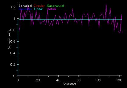
Create shapefile of points convert to point coverage. Krig these points and attach print-out of variogram and interpret.

To do this you open jump, create three columns and 300 rows. Name the first one latitude, the second one longitutde, and use the same formula to create each.

Type 100, click on X, select random uniform.

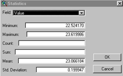
For the z value column the numbers should be normal distribution with a mean of 20 and a standard deviation of 3. The formula should be as follows,

Type 20 choose + select random normal choose + type 3.

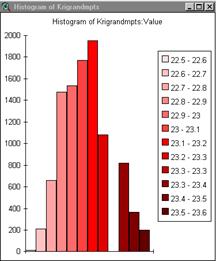
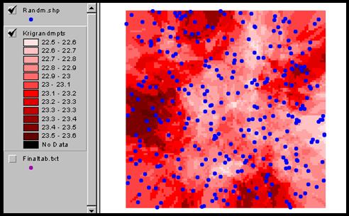
Add the table to a project in ArcView then under select add event theme. After having the help of six classmates for nearly an hour I still don’t know how the shapefile is converted to a coverage. I only know that it finally worked. The display in arcplot never did. However, the display will run in ArcInfo.Grid once arcplot is closed. So, big surprise, the semivariogram is completely flat because it was made from data that is completely random. No correlation. The kriged points are displayed in ArcView and although it seems to have some clustering of higher values, the range is so small that the effect is not significant.